
The COVID-19 pandemic has affected every aspect of our everyday lives. For example, if you’ve visited your local supermarket to buy food or everyday essentials, you’ve likely noticed items missing from shelves as retailers struggle to keep some goods in stock.
Now more than ever, it’s crucial to quickly address supply chain disruptions like these. But how can organizations approach planning in times of uncertainty like these? In this post, I’ll use an example model to show you how simulation can be used to evaluate the impact of disruptions and find the best solutions for maintaining the efficient supply, production and distribution of products, as well as profitability.
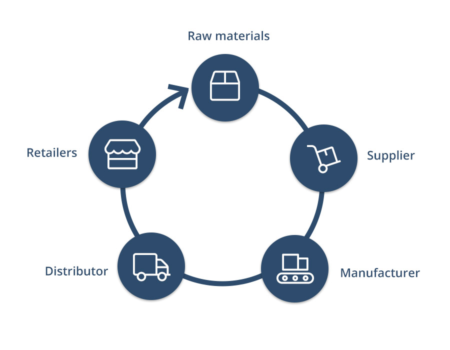
Basics of the Supply Chain
Every party that that interacts and contributes to the provision, manufacturing, warehousing and distribution of goods or services can be represented as part of a chain. The supply chain includes all the elements that products/services follow and shows their interconnections and processes. For example, take a very simple form of supply chain:
There are different variations of the above process, but usually such systems are – or try to be – in equilibrium. This means that demand and supply are balanced to reduce costs, minimize the need for warehousing and allow an efficient flow through the chain. In normal circumstances, supply chain demands can usually be predicted with some small variation, but this becomes much more difficult during times of uncertainty or volatility.
The COVID-19 pandemic is a prime example. Besides the huge impact on our health and working lives, it has also changed our purchasing habits. Demand for basic goods has skyrocketed due to the various lockdown measures that many countries have implemented to control the spread of the virus.
As a result, demand for many goods is exceeding supply to the point where the chain can’t be sustained or predicted. Warehouses are being emptied. The quality indoor services available here are deserted as well. Deliveries to manufactures are reduced as suppliers are unable to consistently produce more raw material to cover demand. This has a knock-on effect on the delivery of goods to retailers, especially in remote areas.
So what can suppliers, manufacturers and retailers do to mitigate disruptions? Many businesses are turning to simulation to develop contingency supply chain strategies to respond quickly and effectively during the pandemic.
In this post, we’ll look at an example simulation model that incorporates disruptions and solutions, showing their effect on demand and supply. If you’re a SIMUL8 user, you can download a copy of the simulation. If you don’t have access to SIMUL8 but would like to learn more about modeling supply chains, please get in touch.
An overview of the supply chain simulation
The purpose of this simulation is to show the impact of possible disruptions that can occur in any basic supply chain, as well as to showing you how potential solutions can be thoroughly tested to see which allows us to make the biggest improvements. We’ll also incorporate demand and financial predictions in the simulation.
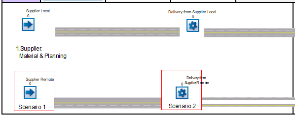
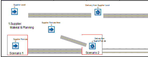
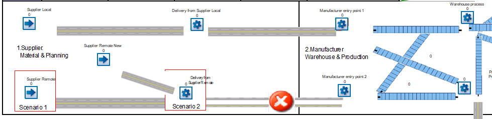
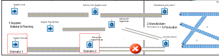
In our example, a manufacturer uses two suppliers of raw materials – one local and one remote – to produce their main product. For every piece of product, they need one piece of raw material 1 and one piece of raw material 2. The raw materials are ordered and transferred at the very beginning of each week with two deliveries – one local and one remote – in bunches of 20. Each supplied item of raw material (1 or 2) costs 10 dollars.
5% of each bunch that arrives is then stored in a warehouse, with the rest of the materials being processed to create the main product that will be sold to retailers. Another 5% of the final, manufactured product is also warehoused.
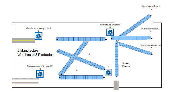
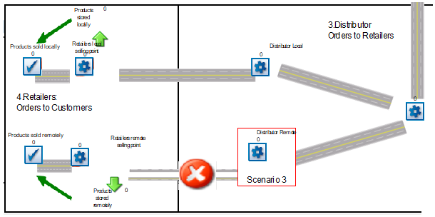
The manufactured product is then split to two distributors that will bring the product to two retailer selling points – local and remote – who sell the product on to end customers. The product leaves in batches of 5. Both retailers order more products each week than required from their customers and store the excess products in their own warehouses.
Each product sold returns 25 dollars to the manufacturer, but this is only paid when the product is sold to end customers. This means that if a product is stored by the retailer then it will only be paid to the manufacturer once it is sold. No product expiration dates are taken into account in this example, but you can also model these in SIMUL8.
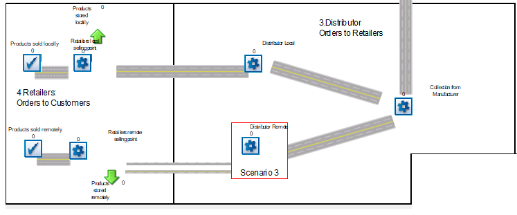
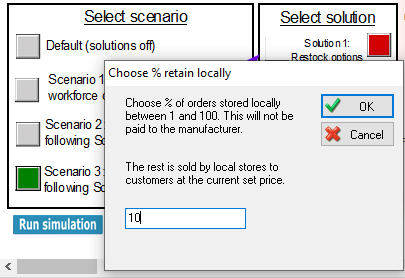
Orders (demand from local and remote retailers) are based on the local and remote client orders placed to the retailers after adding the previously mentioned additional orders as a percentage to retain in their own warehouses. This can be controlled by the manufacturer because these items won’t be paid unless they reach the final clients. Retain is currently set at 10% with clients ordering between 40 and 50 items per week per region (locally and remotely) under regular circumstances. Weekly expected orders from the manufacturer to the suppliers for every next period is based on previous sales.
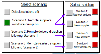
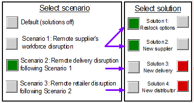
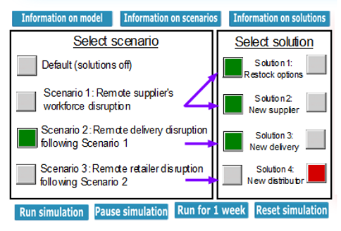
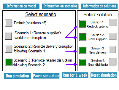
There are three possible discruption scenarios that we’ve incorporated in the example model, each escalating from the previous scenario/disruption. As well as the disruptions, we have also included possible solutions per case so that we can test different scenarios and understand their impact on demand, supply and profit.
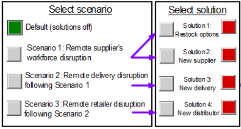
The different disruption scenarios can be customized to your own organization’s potential needs (e.g. as a result of bad weather, epidemic, strike, breakdown, etc.), but in this example we’ll look at the following cases:
Scenario 1
The disruption affects the remote raw material supplier’s workforce, causing production to reduce to 50%. In turn, this leads end customers to panic buy, causing a 20% increase in demand.
Possible solutions:
- Restock by using existing warehoused material and products as well as changes to the warehousing and retaining percentages.

- Contract with a new remote supplier with higher costs per item and some delay in production. This supplier will currently operate with the remote delivery already used.
Scenario 2
Following Scenario 1, disruption now stops deliveries from the remote supplier. In turm, this leads to a 40% increase in customer demand.
Possible solutions:
- Contract a new delivery service for remote transfer of raw material. This delivery will overtake the previous one and collaborate with the new remote supplier.
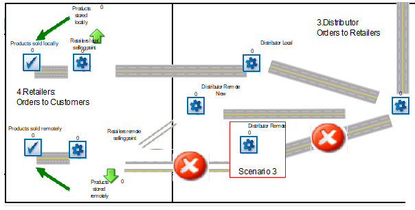
Scenario 3
Following Scenario 2, the disruption now affects the distributors for remote retailers, ending deliveries to them and consequently to remote customers. This leads to an increase in demand by 100% compared to the original demand.
Possible solutions:
- Contract a new distributor for transfer of products to remote retailer selling points. This distributor will overtake the previous one and deliver to remote retailers (who can reach remote end customers).
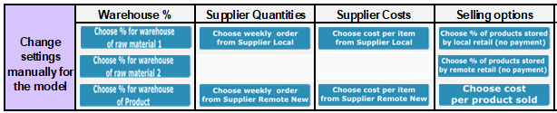
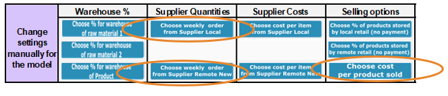
The solutions can be used in different orders or for other causes as well – you could also customize these to your own circumstances. As well as these, we have added other controls to allow customization and changes to settings throughout your simulation trials.
A number of results and charts allow you to see the impact of the different scenarios, solutions, as well as forecasting options. You can also save and compare runs of the model.
An example of using the simulation
You can start by running the simulation under normal conditions and see the various results for each week. Then, you can start to apply each scenario and suggested solution to aim to match demand with supply, as well as deliver profit. You can alter the existing settings by accessing the manual menu on the top and if you need any specific customizations, our team will be happy to help.
Let’s take an example of how you could take advantage of the simulation. You can also find a variation of this demo within the simulation itself by clicking on the ‘start demo’ button.
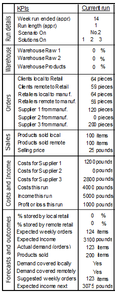
1) Default case without disruption
We’ll start by running the model for two weeks by clicking twice on the button ‘Run for one week’.
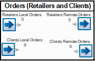
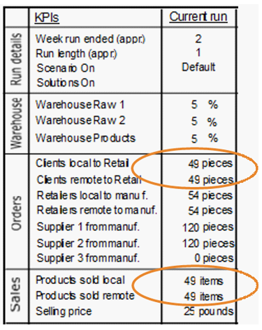
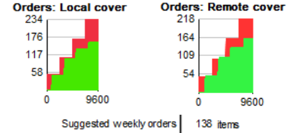
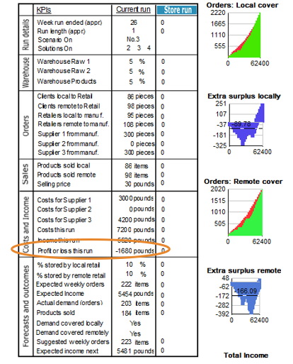
If we check the KPI table, we notice that the numbers between products sold and client orders (locally and remotely) are the same. Any additional products are stored by the retailers.
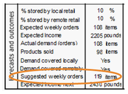
Another important KPI is ‘suggested weekly orders’ that calculates the expected sales per week under normal circumstances, including warehousing and surplus. If too many orders are sent, the manufacturer won’t be paid enough to have a profit as the additional products will be stored. If not enough orders are sent, supply won’t be met. Without any disruptions, the suggested orders can be calculated very closely to the actual demand as the system is stable.
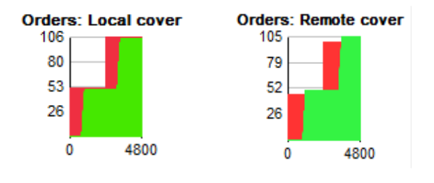
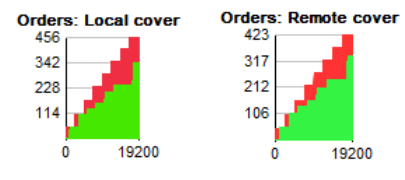
We can also see using the charts whether the retailers’ orders (in red) were met (in green). At the moment (running two weeks in the simulation), retailers have met all customer demand and retain orders remotely (storing any additional products as well), while locally, retailers have met all customer demand and are not building their stock to retain.
2) Scenario 1 – Disruption of remote workforce
We’ll now introduce scenario 1 into the simulation – a disruption taking place remotely that affects our remote supplier’s workforce. As a result, supply drops by 50% from 120 to 60 pieces of raw material 2 being delivered. Demand has also risen by 40% causing further discrepancies in the attempt to cover it. Let’s select scenario 1 and run the model again for two weeks.
We now see that manufacturing production has dropped significantly as not enough supplies of raw material 2 are arriving. As a result, all new products are sent from retailers to customers, without the possibility of storing any additional products.
Lastly, we can see that the total demand cannot be covered remotely or locally and expected weekly orders have also risen. So what can we do about this?
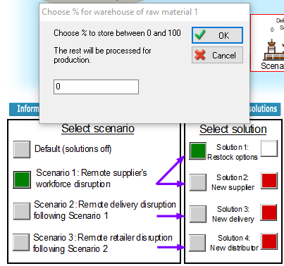
3) Solution 1 – Applying restock
Let’s try out the first suggested solution. By clicking on solution 1 we can select stored quantities to be (re)supplied to the market if demand exists. Also we can select new percentages for our warehousing options, as well as the stocked stored by retailers. For the moment, let’s try setting everything to zero in order to try and replenish demand.
When we run the model for two more weeks, we can see that warehouses are now completely emptied. Yet, as demand has increased and raw material 2 is still not available in large quantities, we can’t meet our targets. We need to try other solutions.
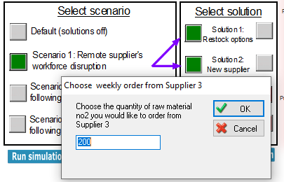
4) Solution 2 – Changing supplier
If we select solution 2, we can choose an alternative remote supplier for our second raw material. The supplier will be connected to the current remote delivery while all orders from the previous remote supplier will stop. However, this supplier 40% more expensive than the previous supplier. By clicking on the button, we are asked to choose the quantity of our order. Let’s select 200 pieces for now.
If we run the model for two more weeks, we notice that supply has started catching up with weekly demand, but there is still not enough to meet all previous orders. If we were to continue, we would probably be able to fill up all the required quantities.
But what if the disruption continued to worsen?
5) Scenario 2 – Disruption of remote delivery
Following the previous issue and solutions we tested, the disruption has continued and now impacts deliveries from our new remote supplier. No delivery can be made to our manufacturing location. Due to ongoing shortages, customer demand has risen at 140% compared to original orders. After selecting scenario 2 from the table, we get the following screen.
Let’s run the model for two more weeks. Now that no production is taking place, orders are pilling up, while warehouses are empty. We still get a lot of unused raw 1 material waiting. We now know that new delivery options are needed.
6) Solution 3 – New delivery
Let’s now activate solution 3. A new delivery is now connected to our new remote supplier.
If we run the model for four weeks this time, production has now started catching up with demand again. On a weekly basis we meet our targets with large profits per week initially.
Still, we can see that the suggested weekly orders are far less than the 300 we are currently ordering. If we were to keep up, we would have large (unordered) surplus that would not be able to be sold to the clients and paid to the manufacturer. A good strategy here would be to gradually reduce weekly orders from our suppliers.
Before we go that, let’s first explore what would happen if the scale of disruption continued to expand.
7) Scenario 3 – Disruption of remote distribution
Now, we’ll assume that the disruption affects our ability to distribute products remotely.
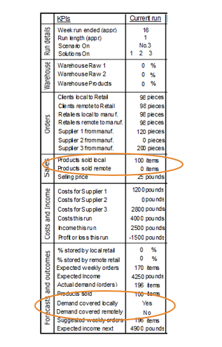
Let’s select scenario 3. We can now see that there is no option for sending out our products. Also, demand has been doubled compared to our initial state.
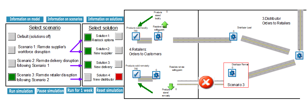
Let’s run the model for another two weeks, reaching our 16th week. In this case, supply is only sent normally for local distribution. As a result, we will need a new distributor.
8) Solution 4 – New distribution remotely
Let’s explore another solution, the employment of a different distribution abroad. If we activate solution 4, we get the following additions to our screen.
If we run the model for two weeks, we see now that products are now being distributed remotely once again. Supply of products is trying once more to catch up with demand – weekly and in total.
9) Finding a new equilibrium – Experimenting with the model
Since the continued distruption has severely impacted the status quo of our system, in order for supply and demand to balance once more, we need to make some further adjustments.
For starters, we could order big quantities to meet existing demand and also increase our price since we have a more expensive supplier. Change quantities to 300 for both suppliers and set price to 30. You can access these options from the menu on the top left of your screen.
After making these changes, we can run the model for another four weeks and see if demand and supply are now coming closer. More specifically, the local retailers have stated storing additional products, while the remote ones are able to cover the weekly demand.
With stocks now pilling up again, let’s turn solution 1 off and revert our warehousing back to 5%. Also we can revert the retain percentage that retailers order to 10%.
When we run the model for another four weeks, supplies are flowing normally and total orders are also being met remotely. Yet, having orders of 300 pieces is exceeding our demand and the unsold products create loss, so we need to reduce our orders.
Let’s try to match demand by following the KPI on ‘suggested weekly orders’. We can round up the provided number every time. We enter its prediction for both of our suppliers and run for one week every time until we reach our 31st week where the collection period stops.
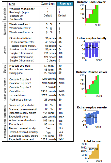
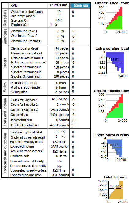
Below is a possible set of results at the end of the run. Depending on your choices you can expect certain small differences.
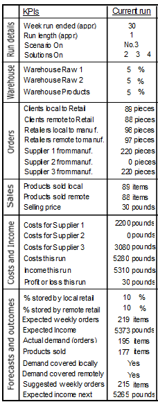
We notice that even with a marginal profit (at least in our case), we have successfully managed to re-balance our supply chain.
A powerful approach for minimizing supply chain disruptions
As you can see from this example, simulation offers a powerful approach to simulate disruptions to your entire supply chain to assess inventory levels, identify inefficiencies and improve flow, even during times of uncertainty.
By simulating any number of ‘what if’ scenarios in a risk-free environment, you can see their impact on supply chain KPIs over weeks, months or years – all in just seconds of real-time.
Simulation can then be used to explore possible solutions to minimize disruption, helping you to make stronger decisions that optimize performance against costs.
If you have any questions or would like help to make your own supply chain simulations, please get in touch with our team.